Module 13: Functions

Amy Winter

Zane Billings

Learning Objectives

After module 13, you should be able to:

Create your own function

Writing your own functions

So far, we have seen many functions (e.g., c(), class(), mean(), tranform(), aggregate() and many more

why create your own function?

to cut down on repetitive coding
to organize code into manageable chunks
to avoid running code unintentionally
to use names that make sense to you

Writing your own functions

Here we will write a function that multiplies some number (x) by 2:

times_2 <- function(x) x*2

When you run the line of code above, you make it ready to use (no output yet!) Let’s test it!

times_2(x=10)

[1] 20

Writing your own functions:

Adding the curly brackets - { } - allows you to use functions spanning multiple lines:

times_3 <- function(x) {
  x*3
}
times_3(x=10)

[1] 30

Writing your own functions: `return`

If we want something specific for the function’s output, we use return(). Note, if you want to return more than one object, you need to put it into a list using the list() function.

times_4 <- function(x) {
  output <- x * 4
  return(list(output, x))
}
times_4(x = 10)

[[1]]
[1] 40

[[2]]
[1] 10

Function Syntax

This is a brief introduction. The syntax is:

functionName = function(inputs) {
< function body >
return(list(value1, value2))
}

Note to create the function for use you need to

Code/type the function
Execute/run the lines of code

Only then will the function be available in the Environment pane and ready to use.

Writing your own functions: multiple arguments

Functions can take multiple arguments / inputs. Here the function has two arguments x and y

times_2_plus_y <- function(x, y) {
  out <- x * 2 + y
  return(out)
}
times_2_plus_y(x = 10, y = 3)

[1] 23

Writing your own functions: arugment defaults

Functions can have default arguments. This lets us use the function without specifying the arguments

times_2_plus_y <- function(x = 10, y = 3) {
  out <- x * 2 + y
  return(out)
}
times_2_plus_y()

[1] 23

We got an answer b/c we put defaults into the function arguments.

Writing a simple function

Let’s write a function, sqdif, that:

takes two numbers x and y with default values of 2 and 3.
takes the difference
squares this difference
then returns the final value

functionName = function(inputs) {
< function body >
return(list(value1, value2))
}

sqdif <- function(x=2,y=3){
     output <- (x-y)^2
     return(output)
}

sqdif()

[1] 1

sqdif(x=10,y=5)

[1] 25

sqdif(10,5)

[1] 25

Writing your own functions: characters

Functions can have any kind of data type input. For example, here is a function with characters:

loud <- function(word) {
  output <- rep(toupper(word), 5)
  return(output)
}
loud(word = "hooray!")

[1] "HOORAY!" "HOORAY!" "HOORAY!" "HOORAY!" "HOORAY!"

Using functions with `aggregate()`

You can apply functions easily to groups with aggregate(). As a reminder, we learned aggregate() yesterday in Module 9. We will take a quick look at the data.

head(df)

  observation_id IgG_concentration age gender     slum age_group seropos
1           5772        0.31768953   2 Female Non slum     young       0
2           8095        3.43682311   4 Female Non slum     young       0
3           9784        0.30000000   4   Male Non slum     young       0
4           9338      143.23630140   4   Male Non slum     young       1
5           6369        0.44765343   1   Male Non slum     young       0
6           6885        0.02527076   4   Male Non slum     young       0

Then, we used the following code to estimate the standard deviation of IgG_concentration for each unique combination of age_group and slum variables.

aggregate(
    IgG_concentration ~ age_group + slum,
    data = df,
    FUN = sd # standard deviation
)

  age_group     slum IgG_concentration
1     young    Mixed         174.89797
2    middle    Mixed         162.08188
3       old    Mixed         150.07063
4     young Non slum         114.68422
5    middle Non slum         177.62113
6       old Non slum         141.22330
7     young     Slum          61.85705
8    middle     Slum         202.42018
9       old     Slum          74.75217

Using functions with `aggregate()`

But, lets say we want to do something different. Rather than taking the standard deviation and using a function that already exists (sd()), lets take the natural log of IgG_concentration and then get the mean. To do this, we can create our own function and this plug it into the FUN argument.

Step 1 - code/type our own function

log_mean_function <- function(x){
    output <- mean(log(x))
    return(output)
}

Step 2 - execute our function (i.e., run the lines of code), and you would not be able to see it in you Environment pane.

Step 3 - use the function by plugging it in the aggregate() function in order to complete our task

aggregate(
    IgG_concentration ~ age_group + slum,
    data = df,
    FUN = log_mean_function
)

  age_group     slum IgG_concentration
1     young    Mixed        0.50082888
2    middle    Mixed        2.85916401
3       old    Mixed        3.13971163
4     young Non slum        0.14060433
5    middle Non slum        2.30717077
6       old Non slum        3.77021233
7     young     Slum       -0.04611508
8    middle     Slum        2.46490973
9       old     Slum        3.52357989

Example from Module 12

In the last Module 12, we used loops to loop through every country in the dataset, and get the median, first and third quartiles, and range for each country and stored those summary statistics in a data frame.

for (i in 1:length(countries)) {
    # Get the data for the current country only
    country_data <- subset(meas, country == countries[i])
    
    # Get the summary statistics for this country
    country_cases <- country_data$Cases
    country_quart <- quantile(
        country_cases, na.rm = TRUE, probs = c(0.25, 0.5, 0.75)
    )
    country_range <- range(country_cases, na.rm = TRUE)
    
    # Save the summary statistics into a data frame
    country_summary <- data.frame(
        country = countries[[i]],
        min = country_range[[1]],
        Q1 = country_quart[[1]],
        median = country_quart[[2]],
        Q3 = country_quart[[3]],
        max = country_range[[2]]
    )
    
    # Save the results to our container
    res[[i]] <- country_summary
}

Function instead of Loop

Here we are going to set up a function that takes our data frame and outputs the median, first and third quartiles, and range of measles cases for a specified country.

Step 1 - code/type our own function. We specify two arguments, the first argument is our data frame and the second is one country’s iso3 code. Notice, I included common documentation for

get_country_stats <- function(df, iso3_code){
    
    country_data <- subset(df, iso3c == iso3_code)
    
    # Get the summary statistics for this country
    country_cases <- country_data$Cases
    country_quart <- quantile(
        country_cases, na.rm = TRUE, probs = c(0.25, 0.5, 0.75)
    )
    country_range <- range(country_cases, na.rm = TRUE)
    
    country_name <- unique(country_data$country)
    
    country_summary <- data.frame(
        country = country_name,
        min = country_range[[1]],
        Q1 = country_quart[[1]],
        median = country_quart[[2]],
        Q3 = country_quart[[3]],
        max = country_range[[2]]
    )
    
    return(country_summary)
}

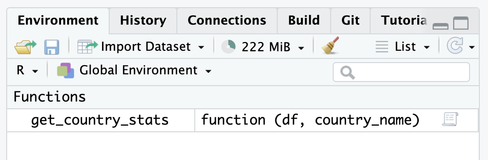
Step 2 - execute our function (i.e., run the lines of code), and you would not be able to see it in you Environment pane.

Step 3 - use the function by pulling out stats for India and Pakistan

get_country_stats(df=meas, iso3_code="IND")

  country  min    Q1 median      Q3    max
1   India 3305 30813  47072 74828.5 252940

get_country_stats(df=meas, iso3_code="PAK")

   country min   Q1 median      Q3   max
1 Pakistan 386 2065   3903 13860.5 55543

Summary

Simple functions take the form:

functionName = function(arguments) {
    < function body >
    return(list(outputs))
}

We can specify arguments defaults when you create the function

Mini Exercise

Create your own function that saves a line plot of a time series of measles cases for a specified country.

Step 1. Determine your arguments, which are the same as the last example

Step 2. Begin your function by subsetting the data to include only the country specified in the arguments (i.e, country_data), this is the same as the first line of code in the last example.

Step 3. Return to Module 10 to remember how to use the plot() function. Hint you will need to specify the argument `type=“l” to make it a line plot.

Step 4. Return to your function and add code to create a new plot using the country_data object. Note you will need to use the png() function before the plot() function and end it with dev.off() in order to save the file.

Step 5. Use the function to generate a plot for India and Pakistan

Mini Exercise Answer

get_time_series_plot <- function(df, iso3_code){
    
    country_data <- subset(df, iso3c == iso3_code)
    
    png(filename=paste0("output/time_series_", iso3_code, ".png"))
    plot(country_data$time, country_data$Cases, type="l", xlab="year", ylab="Measles Cases")
    dev.off()
    
}

get_time_series_plot(df=meas, iso3_code="IND")
get_time_series_plot(df=meas, iso3_code="PAK")

Module 13: Functions

Learning Objectives

Writing your own functions

Writing your own functions

Writing your own functions:

Writing your own functions: return

Function Syntax

Writing your own functions: multiple arguments

Writing your own functions: arugment defaults

Writing a simple function

Writing your own functions: characters

Using functions with aggregate()

Using functions with aggregate()

Example from Module 12

Function instead of Loop

Summary

Mini Exercise

Mini Exercise Answer

Writing your own functions: `return`

Using functions with `aggregate()`

Using functions with `aggregate()`